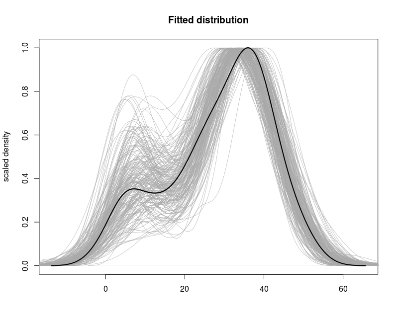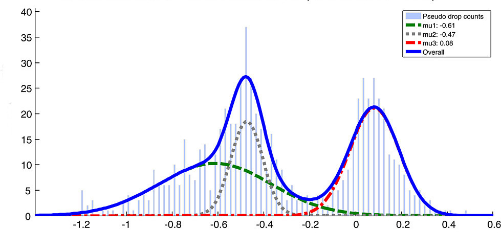
In this project we explore the Gaussian Mixture models. GMMs are universal approximators. This means that any probability density can be approximated to arbitrary precision using mixture of gaussian densities. We saw a glimpse of it in our Hypothesis Testing II project. GMMs are go-to models for unsupervised learning schemes and one of my favorite ML models. In fact, they utilize (usually) EM algorithm, which is an iterative method of estimating statistical parameters similar to and I belive, on par with, backpropagations in Neural nets. In this project we write GMMs from scratch using numpy and stats libraries and compare it against K-means and GMM implementation of Scikit learn.
import numpy as np
from sklearn.datasets.samples_generator import make_blobs
from sklearn.mixture import GaussianMixture
from sklearn.cluster import KMeans
from sklearn.preprocessing import StandardScaler
from sklearn import datasets
import matplotlib.pyplot as plt
import seaborn as sns
sns.set()
from gmmclass import GaussianMixtureClustering
Our implementation resides in gmmclass.py while sklearn has its GaussianMixture class. Below we are comparing sklearns non linear datasets examples to compare and contrast GMMs with Kmeans.
n_samples = 1500
noisy_circles = datasets.make_circles(n_samples=n_samples, factor=.5,
                                      noise=.05)
noisy_moons = datasets.make_moons(n_samples=n_samples, noise=.05)
blobs = datasets.make_blobs(n_samples=n_samples, random_state=8)
no_structure = np.random.rand(n_samples, 2), None

# Anisotropicly distributed data
random_state = 170
X, y = datasets.make_blobs(n_samples=n_samples, random_state=random_state)
transformation = [[0.6, -0.6], [-0.4, 0.8]]
X_aniso = np.dot(X, transformation)
aniso = (X_aniso, y)

# blobs with varied variances
varied = datasets.make_blobs(n_samples=n_samples,
                             cluster_std=[1.0, 2.5, 0.5],
                             random_state=random_state)
# Set up cluster parameters
plt.figure(figsize=(18, 3))
#plt.subplots_adjust(left=.02, right=.98, bottom=.001, top=.96, wspace=.05,hspace=.01)

plot_num = 1

default_base = {'n_neighbors': 10,
                'n_clusters': 3}

dataset0 = [
    (blobs, {'n_clusters': 3}),
    (varied, {'n_clusters': 3}),
    (aniso, {'n_clusters': 3}),
    (noisy_moons, {'n_clusters': 2}),
(noisy_circles, {'n_clusters': 2})]

names = ["blobs","varied","aniso","noisy_moons","noisy_circles"]

for i_dataset, setname in enumerate(names):
    plt.subplot(1, len(names), plot_num)

    X, y = dataset0[i_dataset][0]

    colors = np.array(['#377eb8', '#ff7f00', '#4daf4a','#f781bf', '#a65628', '#984ea3','#999999', '#e41a1c', '#dede00'])

    # normalize dataset for easier parameter selection
    X = StandardScaler().fit_transform(X)

    plt.scatter(X[:, 0], X[:, 1], s=10, color= colors[y] if isinstance(y, np.ndarray) else colors[0])

    plt.xlim(-2.5, 2.5)
    plt.ylim(-2.5, 2.5)
    plt.xticks(())
    plt.yticks(())
    plot_num+=1
    plt.title(setname, size=18)
plt.show()
One can see 5 different examples of interesting non linear datasets with their true classes plotted. Below we use sklearns K-means to evaluate Unsupervised learning. Note that we arent interested in hyperparameter tuning in this project so we will be specifying the number of true clusters for our unsupervised learning model.
plt.clf()
plt.figure(figsize=(18,3))
plot_num = 1
for i_dataset, (dataset, algo_params) in enumerate(dataset0):
    plt.subplot(1, len(names), plot_num)

    X, y = dataset

    # normalize dataset for easier parameter selection
    X = StandardScaler().fit_transform(X)

    algorithm = KMeans(n_clusters = algo_params['n_clusters'])
    algorithm.fit(X)
    y_pred = algorithm.predict(X)

    colors = np.array(['#377eb8', '#ff7f00', '#4daf4a','#f781bf', '#a65628', '#984ea3','#999999', '#e41a1c', '#dede00'])

    plt.scatter(X[:, 0], X[:, 1], s=10, color=colors[y_pred])

    plt.xlim(-2.5, 2.5)
    plt.ylim(-2.5, 2.5)
    plt.xticks(())
    plt.yticks(())
    plt.title("Kmeans: {}".format(names[i_dataset]), size=12)
    plot_num += 1

plt.show()
We note that blobs was best taken care of by the KMeans algorithm. One of the downsides of the Kmeans is the the radius from the cluster center. For varied we observe that the radius likely was large for the orange density center due to which the algorithm attracted non cluster members. This is usually the case when variances differ for different axes (note Aniso dataset above). For other datasets the high non-linearity of the data also shows limitations of the Kmeans scheme.
plt.clf()
plt.figure(figsize=(18,3))
plot_num = 1
for i_dataset, (dataset, algo_params) in enumerate(dataset0):
    plt.subplot(1, len(names), plot_num)

    X, y = dataset

    # normalize dataset for easier parameter selection
    X = StandardScaler().fit_transform(X)

    algorithm = GaussianMixtureClustering(algo_params['n_clusters'])
    algorithm.fit(X, 2000)
    y_pred = algorithm.predict()

    colors = np.array(['#377eb8', '#ff7f00', '#4daf4a','#f781bf', '#a65628', '#984ea3','#999999', '#e41a1c', '#dede00'])

    plt.scatter(X[:, 0], X[:, 1], s=10, color=colors[y_pred])

    plt.xlim(-2.5, 2.5)
    plt.ylim(-2.5, 2.5)
    plt.xticks(())
    plt.yticks(())
    plt.title("GMM : {}".format(names[i_dataset]), size=12)
    plot_num += 1

plt.show()
We observe that our implementation of GMM using Expectation Maximization produced significant improvements over the KMeans. This can be observed in varied and aniso datasets. The latter has difference in variances on axes which is captured by the GMM scheme. For the last two, noisy moons and noisy circles, the GMM method still failed to provide correct clustering. However the story is bit interesting than what it looks. Lets explore the SKlearn libary implementation below.
plt.clf()
plt.figure(figsize=(18,3))
plot_num = 1
for i_dataset, (dataset, algo_params) in enumerate(dataset0):
    plt.subplot(1, len(names), plot_num)

    X, y = dataset

    # normalize dataset for easier parameter selection
    X = StandardScaler().fit_transform(X)

    algorithm = GaussianMixture(n_components=algo_params['n_clusters'])
    algorithm.fit(X)
    y_pred = algorithm.predict(X)

    colors = np.array(['#377eb8', '#ff7f00', '#4daf4a',
                                         '#f781bf', '#a65628', '#984ea3',
                                         '#999999', '#e41a1c', '#dede00'])
    plt.scatter(X[:, 0], X[:, 1], s=10, color=colors[y_pred])

    plt.xlim(-2.5, 2.5)
    plt.ylim(-2.5, 2.5)
    plt.xticks(())
    plt.yticks(())
    plt.title("GMM sklearn: {}".format(names[i_dataset]), size=12)
    plot_num += 1

plt.show()
Above are the result of clustering with Sklearns native GMM model.We find similar imporvements from KMeans in varied and aniso dataset while limitations in noisy moon and noisy circles dataset respectively.
Note that while we stared off agnostic to number of clusters, we can find the optimal number of clusters (K) as the value that minimizes the Akaike information criterion (AIC) or the Bayesian information criterion (BIC).
plt.clf()
plt.figure(figsize=(18 , 20 ))
plot_num = 1
for i_dataset, (dataset, algo_params) in enumerate(dataset0):
    plt.subplot(len(names),2, plot_num)

    X, y = dataset

    # normalize dataset for easier parameter selection
    X = StandardScaler().fit_transform(X)

    algorithm = GaussianMixture(n_components=algo_params['n_clusters'])
    algorithm.fit(X)


    n_components = np.arange(1, 40)
    models = [GaussianMixture(n, covariance_type='full', random_state=0).fit(X) for n in n_components]
    plt.plot(n_components, [m.bic(X) for m in models], label='BIC')
    plt.plot(n_components, [m.aic(X) for m in models], label='AIC')
    plt.legend(loc='best')
    plt.xlabel('n_components');
    plt.ylabel("{}".format(names[i_dataset]))
    plot_num += 1

plt.show()

The numbers in the plots above tell a different story. While for datasets 1-3 the optimal clustering is found by the SKlearn GMM class (obvious from the plots),plot 4 and 5 are what is interesting. It seems like the Sklearn GMM model found optimal num clusters to be 8 and 16 for the last two (noisy moon and noisy circles dataset ) respectively. While we know that the real classes are two for the two datasets, lets observe the consequences of GMM specifying a larger cluster number to those datasets below.
As we mentioned in the beginning, GMMs are Universal Approximators. GMms are also Generative. What these two quality mean is that for any distribution, a trained GMM model is capable of replicating the data from a distribution. Below shows the generative quality of Sklearns GMM for noisy moon and noisy circles dataset respectively, which although the number of classes were larger than ground truth, the effect of larger class number allowed the GMM to fit the non linear behavior appropriately. We finally compare the generative quality of GMM with actual classes as ground truth vs the optimal BIC/AIC classes above.
plt.clf()
plt.figure(figsize=(18, 30))
plot_num = 1
best_params = [12, 20]
for i_dataset, (dataset, algo_params) in enumerate(dataset0[3:]):
    plt.subplot(len(names), 2, plot_num)

    X, y = dataset

    # normalize dataset for easier parameter selection
    X = StandardScaler().fit_transform(X)

    algorithm = GaussianMixture(n_components=algo_params['n_clusters'],covariance_type='full')
    algorithm.fit(X)
    Xold, yold = algorithm.sample(1000)
    plt.scatter(Xold[:, 0], Xold[:, 1])
    plt.xlim(-2.5, 2.5)
    plt.ylim(-2.5, 2.5)
    plt.xticks(())
    plt.yticks(())
    plt.title("GMM Samples: {}, n_clusters={}".format(names[3+i_dataset],algo_params['n_clusters'] ), size=12)

    plot_num += 1
    plt.subplot(len(names),2, plot_num)

    algorithm_best = GaussianMixture(n_components=best_params[i_dataset],covariance_type='full')
    algorithm_best.fit(X)

    Xnew, y_new = algorithm_best.sample(1000)
    plt.scatter(Xnew[:, 0], Xnew[:, 1])
    plt.xlim(-2.5, 2.5)
    plt.ylim(-2.5, 2.5)
    plt.xticks(())
    plt.yticks(())
    plt.title("GMM Samples: {}, n_clusters={}".format(names[3+i_dataset],best_params[i_dataset]), size=12)

    plot_num += 1

plt.show()