Nietzsche, in the premise of Thus Spoke Zarathustra, stated Eternal Return, an idea that all things in the universe will recur and all events in one’s life will repeat again, and again, ad infinitum1. Nietzsche’s world was a deterministic one, Newtonian, with tangible objects, and countable sets. Hence, he viewed his universe like a deck of cards, bound to return to a particular shuffle infinitely on infinite shuffles. But all recurrences need not be perfectly self similar. Far older eyes have imagined universes in kalpas, forever repeating but never quite exactly while the current scientific models view them all in parallel, where each universe just slightly differs from the other. How then are such universes made possible?
This is the third post in the series and 3 is linked to chaos2. However, stepping back a little, I had forever wondered that with all the triumphs in science, with technology to reach the moon and back, predict the spin of an electron correctly to 14 decimal places, why couldn’t we predict if it were to rain on an afternoon? This had made me cognizant of large gaps between some areas of applied & theoretical sciences. Then one day, I stumbled upon a lecture that argued chaos being is a prime example where reduction failed. I then started noticing concepts of chaos emerging everywhere (more like RAS at work than synchronicities), finally coming across some recent studies in chaotic models of the universe, which did it for me. From then on, I needed to know more. Hence, this blog is my meditations in chaos. We will start out exploring what it means for things to be chaotic. We will test conventional methods to predict chaos, note their limitations and finally attempt to see if a class of neural networks with memory based learning units such as LSTMs can help predict behavior of some simple chaotic systems.
Theory
Chaos can be summarized as a aperiodic long term behavior of a deterministic system with sensitive dependence to initial conditions3. Aperiodicity implies lack of rigid temporal structure while sensitivity to initial conditions implies that any small changes in the earlier states of the system will result in exponentially large differences in the later states. Finally, deterministic implies no randomness is allowed in inputs. We will scrutinize each feature from the lens of four 1-D functions below:
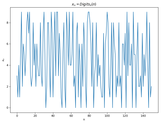
y = sin(\omega t), t \in \mathbf{R}, \omega \in \mathbf{R^+}, \hspace{10mm} \text{(1)}x_n = Fib(n) \text{ mod } p, n \in \mathbf{N}, p \text{ is prime} \hspace{10mm} \text{(2)}x_{n+1} = \lambda x_{n} (1-x_n), n \in \mathbf{N}, \lambda \in \mathbf{R^+} \hspace{10mm} \text{(3)}x_n = Digit_{\pi}(n), n \in \mathbf{N} \hspace{10mm} \text{(4)}
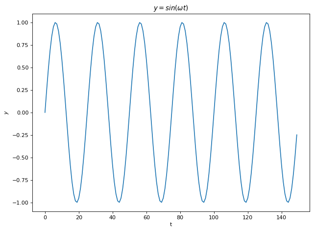
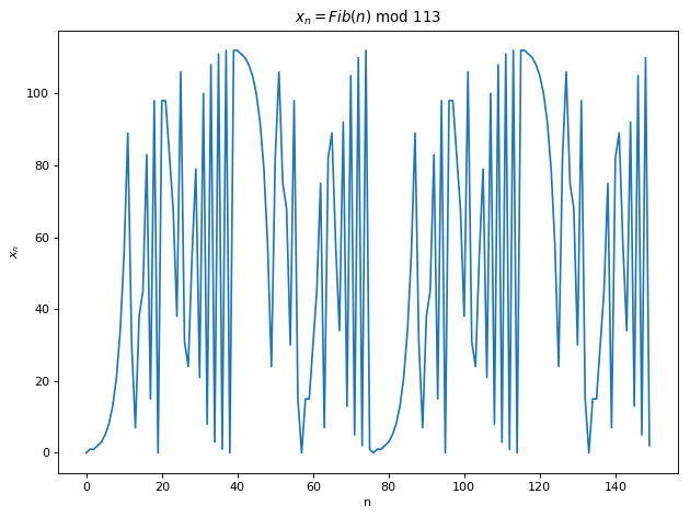
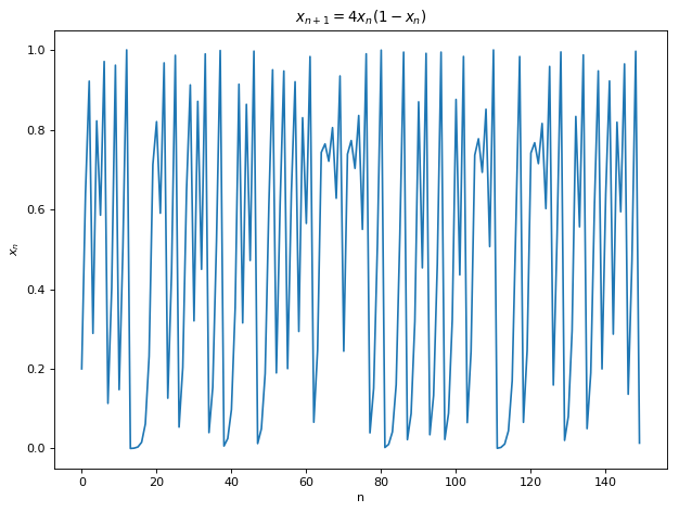
Eq 1 is the sine function. Lets set the frequency f = \omega / 2\pi = 0.04 for the upcoming experiments. Eq 2 gives the n^{th} Fibonacci number modulus a prime number, let p = 113. Eq 3 is the logistic map and we let \lambda = 4 and the initial value x_0 = 0.2. Eq 4 is an unknown function that prints out the n^{th} digits of Pi for a given n. Eq 1 is a textbook periodic while Eq 3 with \lambda = 4 is a textbook chaotic function. We don’t know whether Eq 2 and Eq 3 are chaotic. The plot of f(x) \text{ vs } x for the 4 equations can be seen below. Note that we will use the term map and function interchangeably in this blog treating discrete iterations as continuous time in some of the plots below. While we are incorrect in a strict mathematical sense, I believe this approach is justified when our analysis tools are all computational and our ethos mostly experimental.
Fig 1
Fig 2
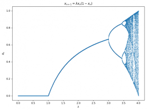
The Logistic map (Eq 3) turns out to be a simple model for many real-life dynamics such as population growth models, predator-prey dynamics, Josheption junctions, etc4. Chaos can be observed in the Logistic map when we plot the roots wrt parameter \lambda. For example, let R_{\lambda} be the solutions to \lambda x_{n}(1-x_{n})=0. R_{\lambda} \text{ vs } \lambda for 0 \le \lambda \le 4 is plotted. One can note that the function converges to one root x^* \text{ for } 0 \le \lambda \le 3 while the solutions bifurcate to 2 roots in the range 3 \le \lambda \le 3.45 and so on. At \lambda \ge 3.57, we observe onset of chaos and emergence of many unstable roots4. From Fig 2 its clear that a simple function such as Eq 3 can exhibit highly complex behavior.
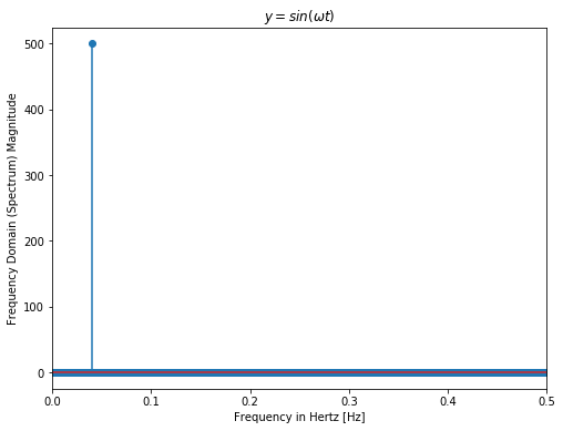
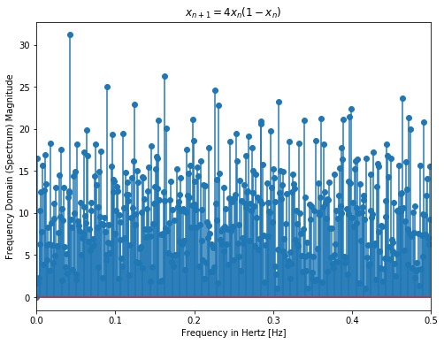
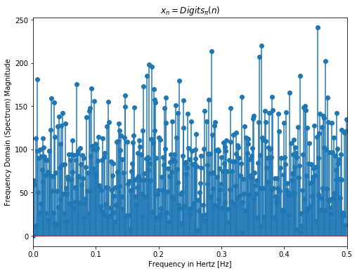
We try to visualize periodicity in our 4 functions in the Fourier domain. Below shows the Discrete Fast Fourier Transform (DFFT) of the first 1000 samples of each function. Sine function as expected has a sharp peak at its frequency = 0.04 i.e its periodic with T = 25 which can be observed in Fig 1 above. Meanwhile one can notice multiple frequencies in other functions. For Eq 2, it looks as if some frequencies are affecting the function more while others negligibly. For Eq 3 and Eq 4, there is somewhat even distribution of frequencies with large fft coefficients. Even though the periodicity is clear for the sine function, from Fourier transforms only, we are unable to ascertain the periodicity of other functions.
Fig 3
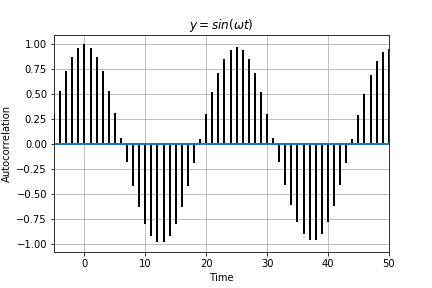
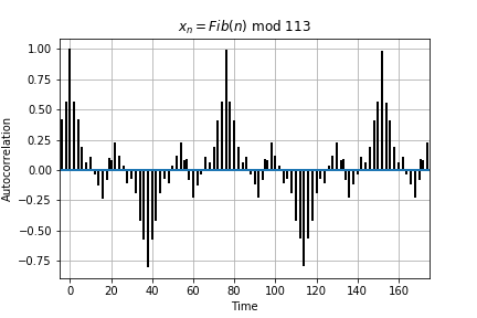
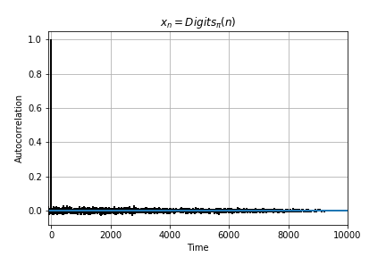
Below is the autocorrelation plots for the 4 functions. Autocorrelation or self-convolution is done in the Laplace domain (here for the amazing Fourier and Laplace connection). From autocorrelation plots we can clearly see that Eq 2 is self similar (autocorrelation approximately 1) for t somewhere near 70. In fact, we find that f(t) = f(t + 76) for Eq 2. Hence, Eq 2 is not chaotic and has periodicity T =76. For Eq 3 and Eq 4, no such autocorrelation is observed (10000 samples is the largest Python allows for acf).
Fig 4
2. Sensitivity to Initial Conditions:
We are at the heart of the matter. Newtonian determinism implied that perfectly calibrated inputs would give rise to perfectly certain outputs. Such determinism led to a model of clockwork universe. However, Poincaré was earliest to point out a flaw in the model when he added the Moon in the Earth-Sun dynamics where the Newtons’ Law of Gravitation failed, the problem of scientific ménage à trois.
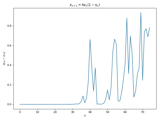
Sensitivity to initial conditions is crucial to chaos and is often termed as the butterfly effect. It essentially means that no matter how close two points start out with, their pathways eventually diverge. Therefore, one cannot naively treat tiny differences in inputs as noise, which stabs in the heart of reductive approaches such as linear and non-linear regressions. Below shows the plots showing sensitivity to initial conditions for Eq 3. Plot 1 & 3 show the diverging paths due to slight differences in starting points. Plot 2 & 4 show the absolute differences in the paths in which one can observe tiny differences initially that become large after a certain time.
Fig 5
Such sensitivity to initial conditions is measured in terms of Lyapunov exponents. The idea behind Lyapunov exponents is similar to the idea of a derivative, we measure the change in dependent variable with respect to small change in the independent variable. Here the independent variable is the initial condition and dependent variable is the state of the function at a later time. Strictly, for any two initial conditions (x_{00}, x_{10}), let the state of the system at time t be (x_{0t}, x_{1t}) = (x_{00}+dx_{0t}, x_{10}+dx_{1t}), we define \delta_t = |x_{0t}-x_{1t}| as the divergence between the two trajectories at time t. The Lapunov exponent is then defined4 long term logarithmic rate of divergence of two trajectories: \sigma = \lim_{t\to\infty}\frac{1}{t}ln(\frac{\delta_t}{\delta_0}) = \lim_{t\to\infty}\frac{1}{t}\sum_{i=0}^{t-1}ln|f'(x_i)| \hspace{10mm} \text{(5)} Note that there will be n Lyapunov exponents for n-dimensional maps. Its also enlightening to rewrite Eq. 5 as \delta_t^{\varepsilon} = \delta_0e^{\sigma t}\hspace{10mm} \text{(6)} where \delta_t^{\varepsilon} = |x_{0t}-x_{1t}|\le \varepsilon for some error tolerance \varepsilon \in \mathbf{R^+} from which one can compute the Lyapunov timet_{\varepsilon} such that \delta_t \le {\varepsilon}. Using Eq 5, we compute the Lyapunov exponent for Eq 3 to get \sigma \approx 0.693 . This value plugged in to Eq 6 provides t_{\varepsilon} \approx 7 and t_{\varepsilon} \approx 37 for \varepsilon = 0.1 \text{ and } \delta_0 = \text{1e-3}, \delta_0 = \text{1e-12} , respectively, which aligns with the observation in Fig 5.
3. Deterministic Inputs Indeterminate Outputs:
To me, this is the most exciting concept in the ideas of chaos. We noted earlier that aperiodicity implied lack of rigid temporal structures. From Fig 1 one can note the y-axis values for Eq 3 seem to be random. However, Chaos and Random aren’t the same but they’re close. For example, below are the 20 iterations of the Eq 3:
What we just did above is Symbolic coding of a chaotic function. We then claim that the series resulting from such coding of our Eq 3 indistinguishable from random5. This is an absurd claim. However for all practical purpose its true. So true that its the basis of random number generation in a deterministic system such as a computer, and are called Psuedo-Random Numbers. I suggest you try it out, compare the values with a real random coin toss sequence from Random.org (here of an amazing blog on tests of randomness).
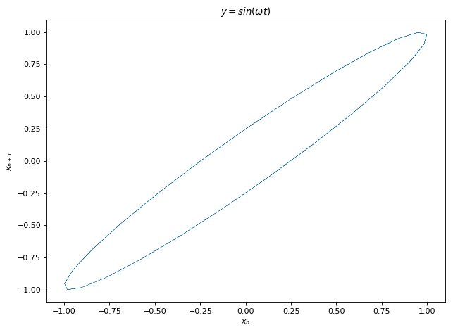
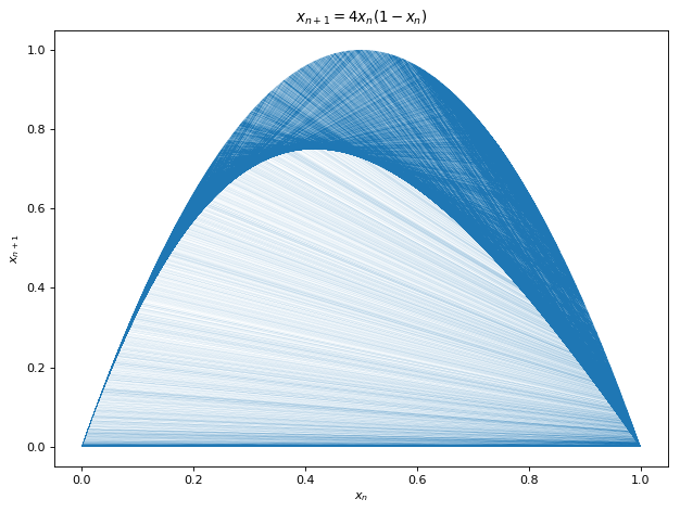
Now you’d have to say, wait a minute, each sample in a coin toss is independent of the previous or next or any other tosses. This is clearly not true for Eq 3 since x_{n+1} depends on x. We can see this in (x_{n},x_{n+1})Poincaré plots below which reveals persistent structures for our four equations. We note the inverted parabola for Eq 3 while a dense discrete network for Eq 4. This should give us the estimate of the complexity of the functions we are tying to learn. Eq 1 and Eq 3 seem easier compared to Eq 1 and especially Eq 4 for function learning due to discontinuities involved in the latter. Finally, since there exist functions that generate pseudo-random numbers with persistent structures before being masked by symbolic codings, could we learn this hidden structure from the series of psuedo-random numbers and win bets on average with computers. We try this out in our experiments.
Fig 6
Learnability
Some notes on learnability before we move to experiments. We know that learning is more than memorization. A perfect memorization fails to generalize to unseen examples and is called overfitting. Learning is more of an encoding. Perfect encoding such as formulae, eg. Newton’s laws, are elegant and generalize very well to unseen data. The idea of reduction is to follow occam’s razor i.e. the simplest formula that describes the phenomenon well enough is chosen. Most of the time, such simple formula describes trends and not individual data points and especially not anomalies, which are usually treated as noise. In our case, we will treat our signal as void of noise. We want to be able to encode such a way that we describe individual data points well. Hence, we will try to fit individual training points while maintaining testing accuracy and avoiding the overfitting. We are not interested in seasons, but the weather, esp given the weather now and in the past, if its going to rain in an hour, figuratively.
Based on Information Theory, one can also think of encoding as the number of bits it takes to describe something6. Lets take a number 2, it takes two bit to describe it perfectly, while a number 1/3 takes around 5 bits (1 for 1, 2 for 3 and 2 for ‘/’ if its chosen from a set of (+,-,* , / ), etc. Other representations of 1/3 are the string ‘1/3’, '0.\bar{3}', etc. Hence, we can ignore how strings or ints are actually represented in a computer but think of it in terms of information representation6. All rational numbers have finite representation. Almost all irrational numbers have no finite representation and thus no encoding. However, there are some which do, for example, \sqrt{2}. It took me two letters to write it down and communicate perfectly what it is. The same \sqrt{2} written as ‘1.4142135623..’ is not a finite representation. Hence, while the data may seem to be infinite in one representation, it may still have a finite encoding in another representation. So the question is if, from the time series data generated by an irrational number \sqrt{2}, we could learn the function itself, i.e. sqrt().
Btw, any solution to analytic function, if it exists, has finite representation, the representation being the function itself. I’ve chosen \pi for Eq 4. \pi‘s finite representations include the symbol \pi itself, the formula \frac{Perimeter}{2r}, its power series expansions, continued fractions, and others. The idea is that each digit of \pi is not random for the generator function exists, BBP for example, and we want to learn it using function approximators such as neural nets. Finally, you maybe wondering why we are using an irrational number in the analysis of chaotic functions. The symbolic coding such as one we did earlier generates a unique irrational number for a given initial condition, for example 011011100… is binary for some irrational. Hence there is a deep connection between the two and symbolic dynamics are usually enough to understand the dynamics of chaotic systems5.
Experiments
1. Discrete Fast Fourier Transform (DFFT):
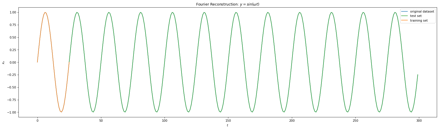
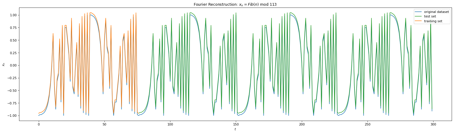
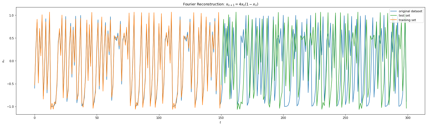
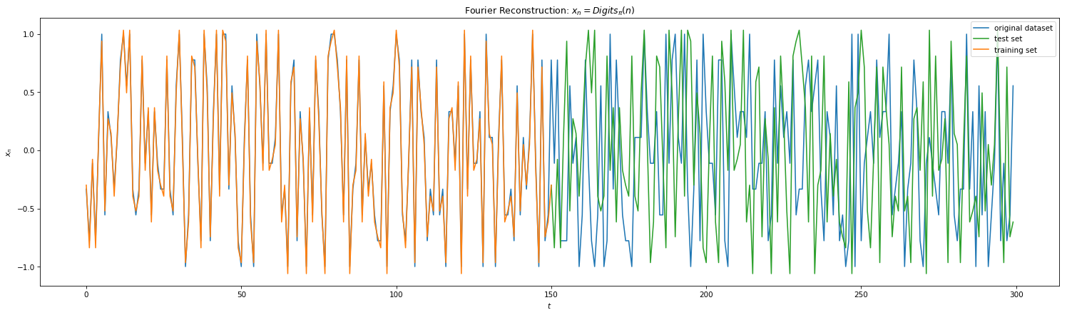
From Fig 3 and Fig 4, we were able to ascertain periodicity of Eq 1 and Eq 2. With finite periods, DFFT is the go-to method for signal reconstruction. Here we initially map our time series in Frequency Domain, filter high order frequencies (noise) if needed and remap the signal back to the time domain. Below shows the results of DFFT for the 4 equations. With minimal training samples of 1 period, we were able to reconstruct the signals quite perfectly for Eq 1 and 2. However, one can notice this method failing for Eq 3 and 4. Due to lack of periodicity, we are forced to choose finite frequencies for reconstruction. This implies that the DFFT method will reconstruct only a subset of the signal which will repeat. Hence, the method fails to generalize right away to unseen data (frequencies).
Fig 7
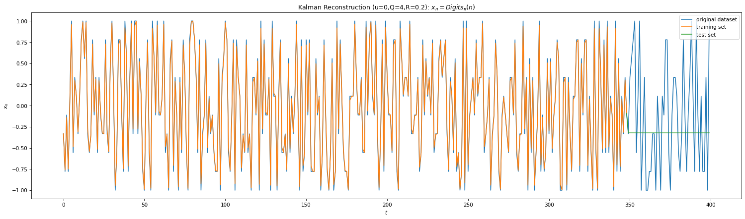
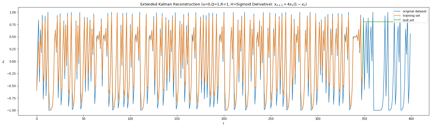
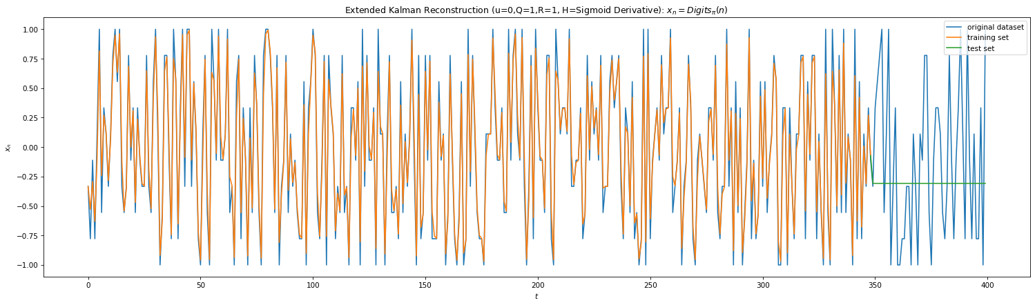
2. Kalman Filters:
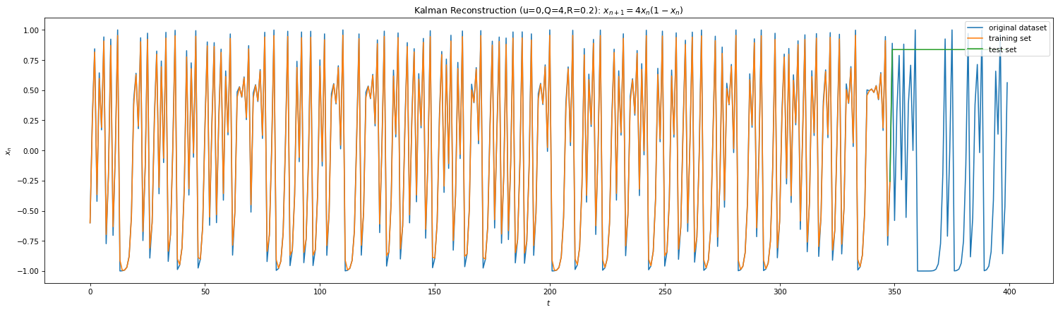
A discrete-time Kalman Filter (KF) is equivalent to a Bayesian belief propagation technique7 and is widely used in engineering. A Bayesian method of inference uses Bayes’ rule to update probability for a hypothesis or estimates as more information becomes available. A belief underlies uncertainties to the hypothesis. Hence, KF is two step algorithm. In the prediction step, estimates of next state of a variable with uncertainties are computed. The state is then measured, with noise, and the prediction estimates are updated using weighted averages. The underlying model is HMM (here for an amazing lecture on Bayesian networks).
Fig 8
Above shows the predictions of the KF for Eq 3 & 4. We’ve also plotted the performance of Extended Kalman filters (EKF). KF is linear in state space and doesn’t capture non-linear dynamics well. One way to get around this is to linearize the dynamics around the weighted mean which leads to EKF. However in our case, we measure at each iteration and the dynamics is linear between two measurements, hence EKF & KF performs similar. Due to lack of analytical understanding for Eq 4, I’ve ad hoc used derivative of the sigmoid as the non-linear Jacobian.
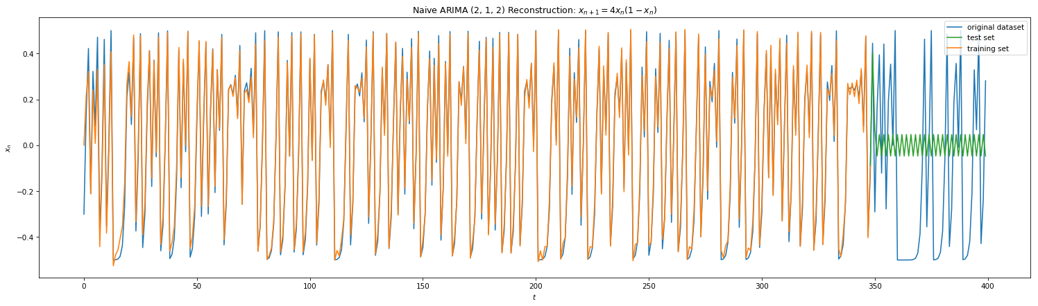
3. AutoRegressive Integrated Moving Average (ARIMA):
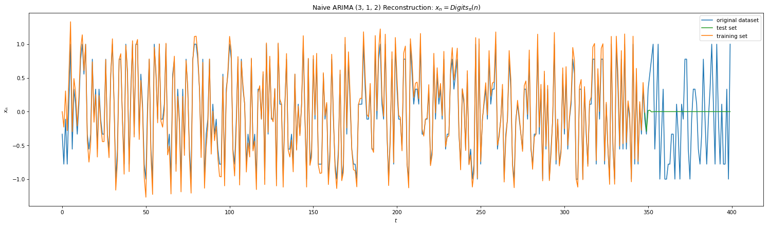
KF worked well for single step predictions. However, we would like to peek further into the future. ARIMA uses KF along with other tools: auto-regression (AR), differencing (I) , and moving averages (MA) to model time series in a more robust manner. Auto-regression builds linear regression model by lagging the time-series with itself and is defined by parameter ‘p’. Differencing is a technique where you subtract the timeseries by its previous iteration. The parameter ‘d’ defines the number of time you difference the series to get a stationary model. Moving averaging is where you update the current model with new measurements with decay parameters. Parameter ‘q’ sets the order if the MA. Below is the results of ARIMA on Eq 3 and 4 with params (p,d,q). Note that the SCIPY.stats implementation only allows d < 2 and thus we self create stationary version by differencing ‘l’ times on plots 3 & 4. We note that in both naive and stationary models, the prediction is good to at most 2 steps in the future.
Fig 9
5. Long Short Term Memory (LSTM):
LSTM are a class of Recurrent Neural Networks (RNNs), which are the neural nets with feedback loops. The feedback loop from the RNN helps take the output of previous iteration as a input feature for the current iteration helping the neural network learn time series data such as language, video, stock prices etc. While in principle the network should learn from past experience, RNN fails to learn long term context due to vanishing gradients. The LSTM improves upon RNN’s by utilizing CEC’s that help counteract the vanishing gradients making long term contextual learning feasible8. We will be utilizing the network for chaos prediction.
5.1. The Logistic map
5.1.1. Forecasting & Generalization:
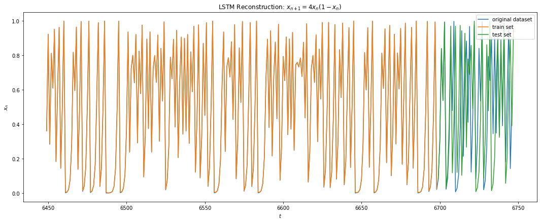
The LSTM regressor architecture9 comprised of 2 layers of Bidirectional LSTM with 4 & 2 units respectively followed by two dense hidden layers of size 8 and 4 units. The activation functions were all Relus and the GD optimized with adam. The cost function used was RMS loss. No dropout were used since the goal was to minimize the training error as much as possible. The dataset used was first 10K samples of the iterations of Eq 3 with x0 = 0.2 with 67% of the data used in training and rest used in testing. A 1 step look-back gave the best results. This makes sense since Eq 3 only depends on its previous recurrence.
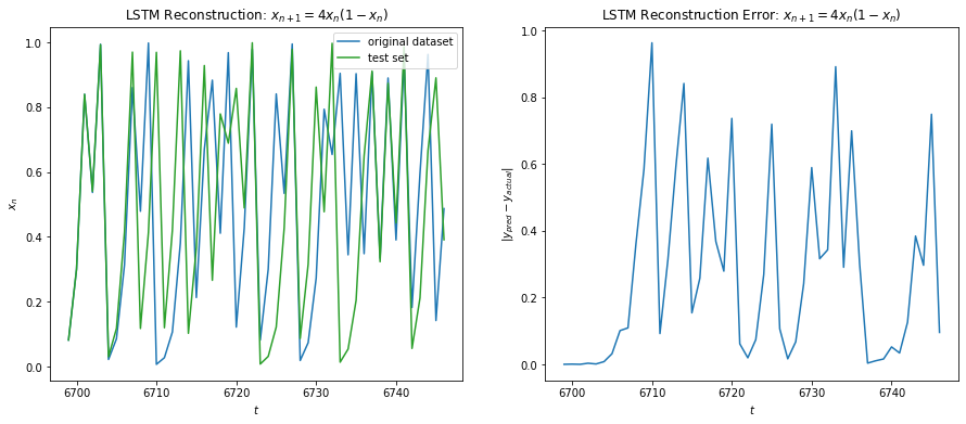
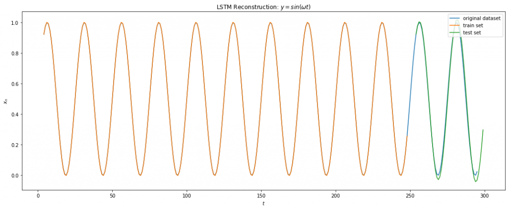
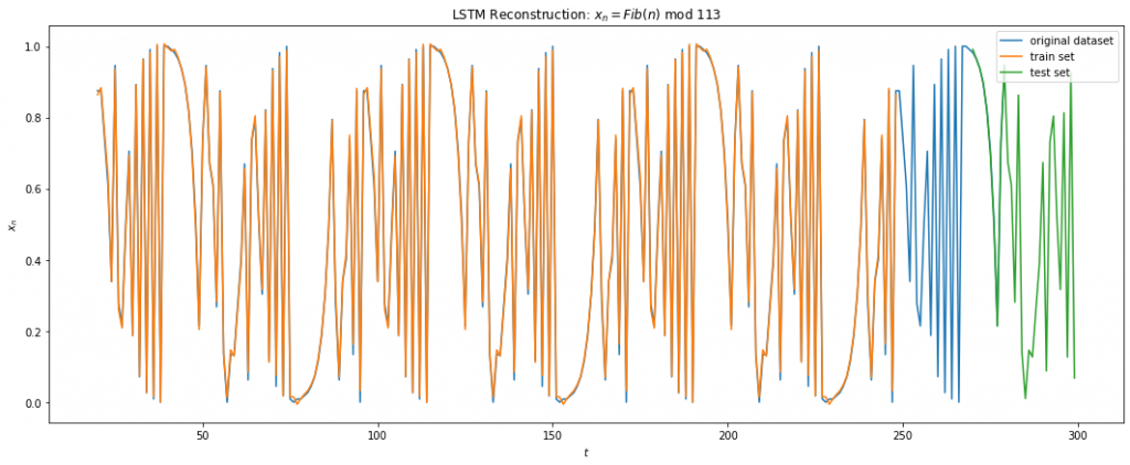
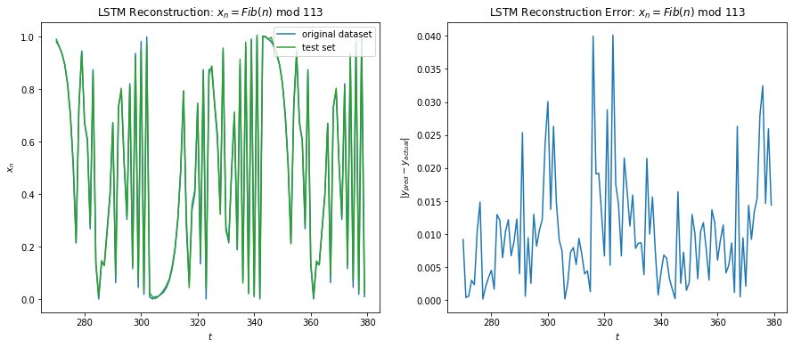
Below shows the results of LSTM on Eq 3. I was able to achieve a training error of 1e-3 on around 1000 epochs. We can see from Fig 10 below that the LSTM fits the function fairly well for the training data. For the test data, we make multi step prediction by taking the last training sample and making the prediction, then taking that prediction and making another one and so on. We see that LSTM does great in multi time step forecasting beyond the training data for about 7 iterations into the future.
Fig 10
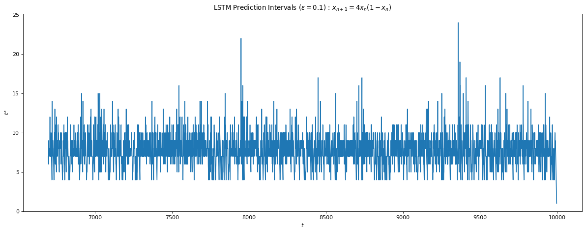
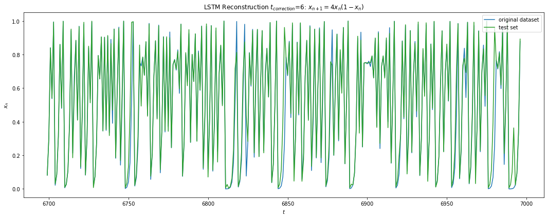
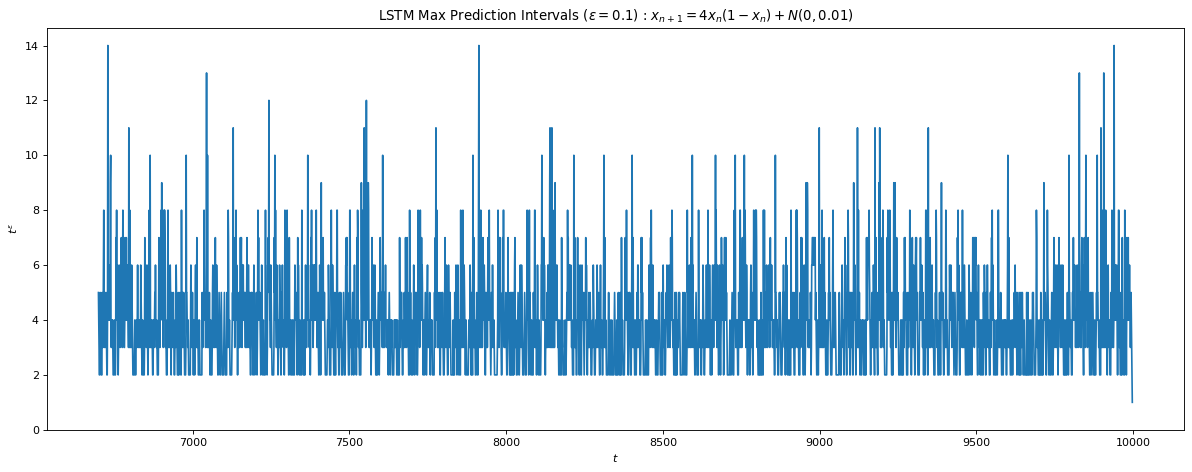
Fig 11 a) shows the maximum iterations before the test error \gt 0.1 for each test sample with average ~ 7.68 iterations. This is consistent with the Lyapunov time we computed for 1e-3 difference in the initial condition signalling the possibility that had we been able to reach a lower training error, the prediction window would increase as well. Fig 11 b) shows a correction scheme where after 6 iterations we correct for the residual error in our predicted path similar to the KF update, which allows the LSTM to predict infinitely into the future.
Fig 11
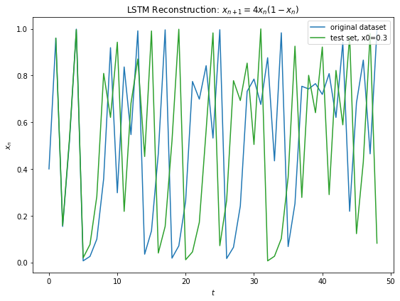
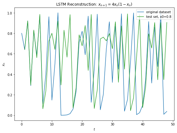
Fig 12 below shows generalization of the learned model to Eq 3 with different initial conditions. Similar prediction window of around 8 iterations is observed before the chaos prevails.
Fig 12
5.1.2. Forecasting with Noise:
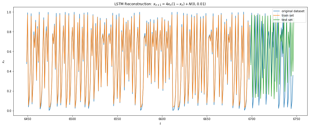
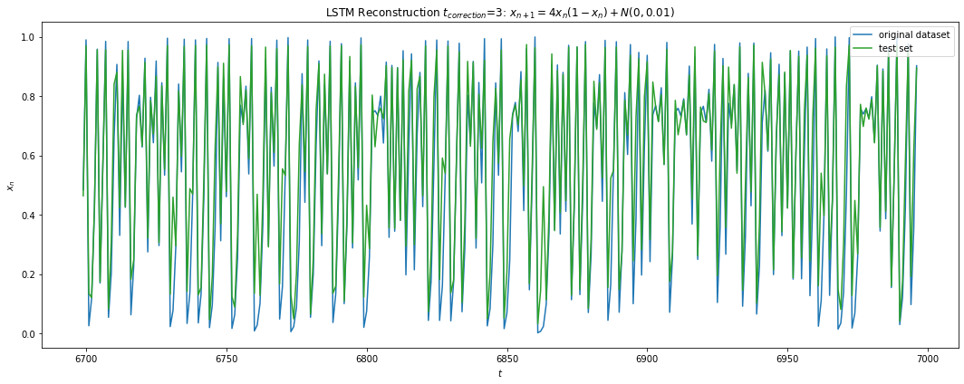
All real life dynamics include noise (sensor noise, precision, etc). We would like to see the performance of LSTM with noisy signal. Here we have added small noise n to Eq 3 such that n is gaussian N(0,0.01) if 0 \le | Eq 3 + n| \le 1 else n = 0. We used the same architecture in 5.1.1 above except that small dropouts were now added to our hidden layers (5% and 1% respectively). Fig 13 shows the prediction performance of LSTM. The minimum training error achieved was around 0.034. Fig 14 a) shows the reduction in the prediction horizon to an average of 4 steps with Fig 14 b) showing consistent reconstruction still possible with correction updates after each t=3 prediction.
Fig 13
Fig 14
5.1.3. Predicting Symbolic Dynamics:
This experiment converted the dataset to binary by thresholding at 0.5 similar to when we discussed the symbolic coding. LSTM classifier was trained with architecture similar to 5.1.1. The max training accuracy achieved was ~0.52 i.e. 52%. While this is great and slightly better than a random guess, the test accuracy was 0.5 and wasn’t significantly different from random for any prediction intervals beyond training. Hence, the PRNG scheme still looks safe with this regard.
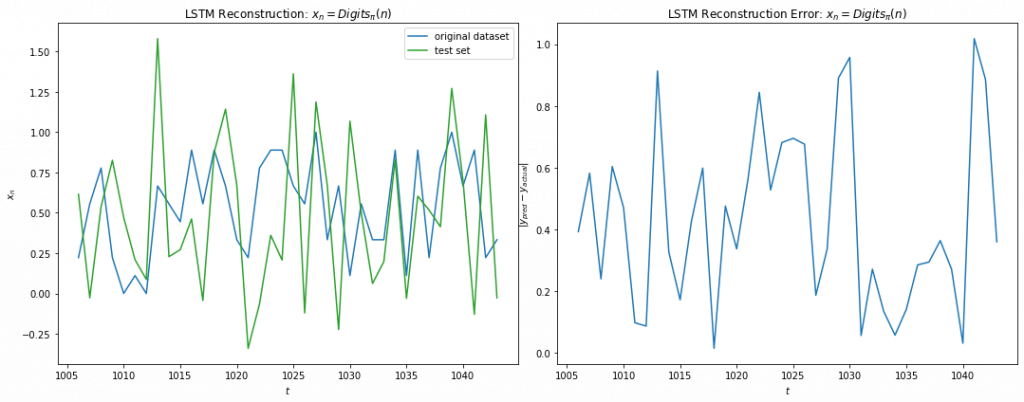
5.2. Digits of Pi
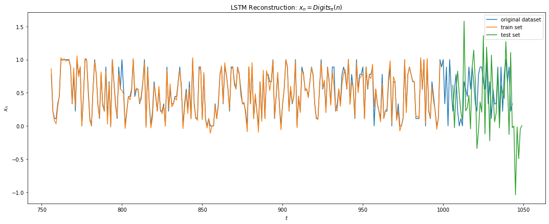
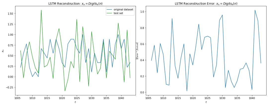
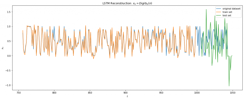
The LSTM regressor architecture comprised of 2 layers of Bidirectional LSTM with 16 & 4 units respectively followed by three dense hidden layers of size 8, 4 and 4 units. The activation functions were all Relus and the GD optimized with adam. The cost function used was RMS loss. No dropout were used. The dataset used was first 1500 samples of digits of Pi scaled to 0-1. 67% of the data was used in training. While the look-back in range 64 to 128 were tested with larger LSTM and hidden units, they failed to converge. A 6 step look-back trained on 4K epochs gave the training error of 0.09 but fails to generalize. Below we note the overfitting on the training set which massive overshoots in the test data. This is most likely Runge’s phenomenon as the LSTM tries to fit the training data will higher order polynomials as it fails to find a low order representation.
Fig 15
As with 5.1.3, I’ve tried to run a LSTM classifier with 10 output nodes predicting the next digit of Pi from the previous values. I was able to get training accuracy of ~0.24 with the testing accuracy was no better than 0.1 for any prediction window and hence, the classifier was no better than random. I’d also noticed the erratic nature of the loss possibly due to the non-continuous nature of the cost function, which did make me appreciate classification as much of a harder problem than regression.
Results
Summary
The LSTM networks were successful at signal reconstruction and multi-step predictions for Eq 1-3. For Eq 3, which is the Logistic map with \lambda = 4, the prediction horizon of the network was about 7 iterations into the future before the test error became \gt 0.1. For the LSTM training error of 1e-3, this is consistent with the Lyapunov time we computed for the initial sensitivity of 1e-3. We were also successful at reconstructing the Logistic map with small added noise with a reduced prediction horizon of 4 iterations into the future. Compared to other conventional methods discussed in the Experiment section, we note that the LSTM was robust for its multi-step prediction. For Eq 4, the network overfitted the data and failed to generalize. However, looking at the dense Poincaré plot of Eq 4 in Fig 6, this was sort of expected.
I hope by now we look at Chaos in a different light. I prefer the word complexity for the word chaos itself has a negative connotation. It could be an artifact of Newtonian determinism mixed with the lack of algebraic techniques to study and predict, but I find physicists hating the concepts of chaos, doing everything to avoid them in the textbooks while engineers trying hard to control with limited success. This limitation just shows the complexity of the dragons we are dealing with, which should be exciting and taken seriously. For what was magic of yesterday is today’s science, and while the aether may have been abolished, the magic still persists in earth, air, water and fire; all with varying degree of chaotic dynamics. And so the challenges of climate change, space travel, geoengineering, nuclear fusion, beating cancer or studying the origins of life, all still seem out of reach. But 21st century science steps up.
References
Notes on the Eternal Recurrence – Vol. 16 of Oscar Levy Edition of Nietzsche’s Complete Works.
Period Three Implies Chaos, Tien-Yien Li and James A. Yorke, The American Mathematical Monthly Vol. 82, No. 10 (Dec., 1975), pp. 985-992
Strogatz, Steven H. 1994. Nonlinear dynamics and Chaos: with applications to physics, biology, chemistry, and engineering. Perseus Books (p. 21, 371, 367) 1994.
Excellent overview of chaos. The graphics and examples work well to describe this difficult concept. I find it refreshing to embrace chaos as an integral aspect of the universe. Respecting the natural world for its complexities instead of shying from the challenge is a critical first step in achieving a better understanding.


June 25, 2020
Excellent overview of chaos. The graphics and examples work well to describe this difficult concept. I find it refreshing to embrace chaos as an integral aspect of the universe. Respecting the natural world for its complexities instead of shying from the challenge is a critical first step in achieving a better understanding.